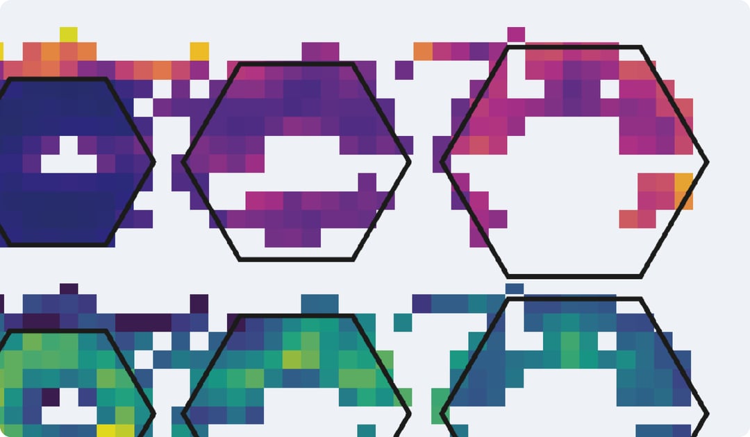
Cathodoluminescence (CL) imaging techniques unveil various properties of materials, such as zonation, deformation, band edge emission, light directionality, defects, and more. In all material types, the emitted CL is the result of physical processes taking place in the material, and so there are time dynamics associated with these emissions. Below, we will highlight how these dynamics can be studied using time-resolved CL.

The temporal dynamics of CL emissions can be measured using one of two time-resolved CL techniques, namely decay trace mapping and g(2) mapping. 

Decay trace

In time-correlated single-photon counting (TCSPC), a short electron pulse is used to bring the material to an excited state. A single-photon detector combined with a time-correlator is then used to detect photons that are emitted from the sample and record the delay between the excitation pulse and the arrival of the photon. By repeating this measurement a large number of times, a decay trace is reconstructed from which the characteristic emission lifetime (tau) can be extracted. This lifetime is typically taken as the time it takes for the emission intensity to drop to e-1 of its initial value.

The lifetime of an emitter is strongly correlated to its material properties, such as recombination rates, doping levels, and defect density. This makes TRCL a great technique for analyzing, for example, semiconductor materials intended for use in optoelectronic and electronic devices. This method can be combined with spatial mapping to image variations in lifetime as a function of position at high resolution. 

g⁽²⁾ mapping

The second time-resolved CL technique is g⁽²⁾  mapping, which measures the autocorrelation function, that is, how the photons emitted from a source are distributed in time. This is particularly important for fundamental studies on quantum systems and their interaction with electron beams as it enables the identification and characterization of single-photon emitters at the nanoscale. Both continuous electron beams as well as pulsed electron beams can be used for g⁽²⁾  measurements. 

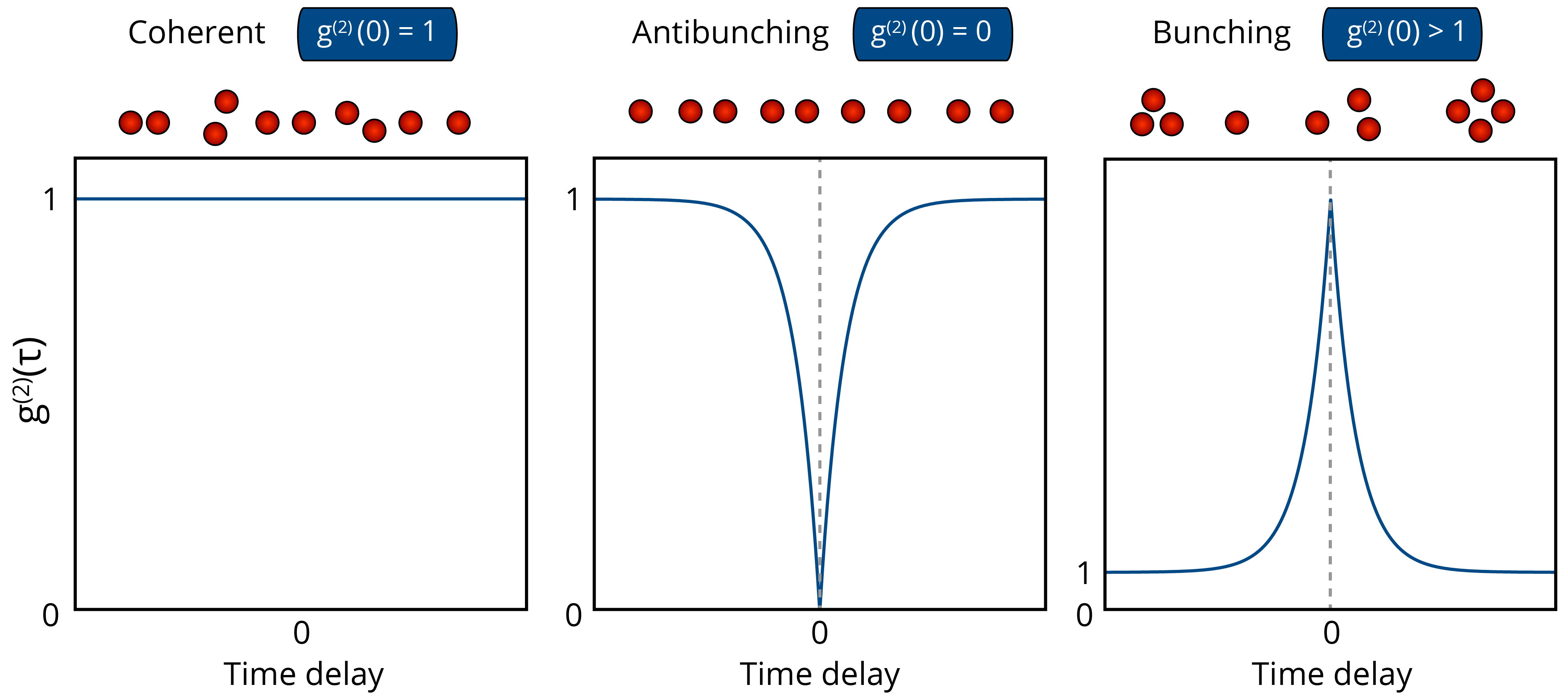
g⁽²⁾ measurements can reveal three characteristic behaviors: coherent, for a coherent source such as a laser; antibunching, for quantum emitters such as NV centers in diamond, single molecules, or quantum dots; and bunching, for incoherent emitters (Figure 1). Additionally, the g⁽²⁾ function can be used to measure the lifetime and the excitation probability of the emitter. High-resolution spatial mapping can also be performed with g⁽²⁾ measurements by scanning the electron beam.

Figure 1: Three characteristic behaviors of emitters, revealed using g⁽²⁾  spectroscopy.

Performing time-resolved CL measurements

Decay trace and g⁽²⁾ measurements can be performed using Delmic's Lab Cube, an additional SPARC Spectral module designed for time-resolved CL imaging. The Lab Cube integrates two configurations into a single system. It's equipped with color filters to measure lifetimes for different transitions within the detection range.

For lifetime mapping, a single photon detector (such as a PMT) detects the photons emitted in every pulse and sends the signal to the time correlator. By repeating the experiment, the exponential decay plot is constructed and the lifetime is extracted. 

For g⁽²⁾ mapping, the Lab Cube uses two single-photon detectors to measure coincidence, as the electron beam is not pulsed. The lifetime plot is built up by repeating the measurement and the characteristic lifetime is extracted from the width of the curve. 

By scanning the electron beam, a spatially resolved lifetime map can be acquired using either technique, enabling the study of lifetime as a function of position on the sample.

Time-resolved CL is a versatile tool that can be successfully applied to a wide range of materials and devices, such as nanostructured semiconductors, phosphors, ceramics, quantum emitters, and even geological materials. To learn more about time-resolved CL, please download our technical note below.